How Rittman Analytics Centralizes SaaS Data Sources using dbt and Google BigQuery

Around this time last year I put together a blog post titled “How Rittman Analytics Does Analytics” in which I went through the tools and delivery approach we used when building analytics solutions for ourselves and our clients using Looker, Google BigQuery, dbt and Stitch.

In that initial blog article I focused more on our Looker dashboards and the framework of KPIs we used for our own internal analytics. In this update to that post I’m going to focus this time on the underlying data warehouse layer and how we use dbt to model, transform and load data into that warehouse using our RA Data Warehouse dbt Framework we’ve recently published for public access, forking and PRs on Github.

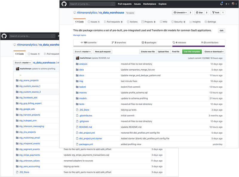
So what does this framework contain, and what problems does it solve for our team of analytics engineers working on our client and internal projects?

What is the RA Warehouse dbt Framework?

The RA Warehouse dbt framework is a set of data models, data transformations and data warehouse dimensional models we use for ingesting, combining and restructuring data from multiple source systems into a conformed, Kimball-style data warehouse using

• Google BigQuery (Standard SQL)
• dbt
• Stitch
• Fivetran (limited support as of now)
• Segment (limited support, but along with Fivetran, on our immediate roadmap to complete

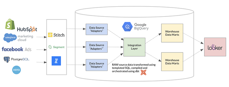
For anyone who’s not so familiar with dbt, it’s an open-source toolkit sponsored by our friends and partners over at Fishtown Analytics that solves the problem of testing, repeatability and modularity of analysts code by bringing the principles of modern software development to the analysts’ workflow.

Our data warehousing framework for dbt tries to solve the problem of how to design your warehouse so that your project doesn’t grind to a halt after you integrate your second, third, fourth data source. It’s been our experience that complexity increases exponentially in data centralization projects as you add more sources into the warehouse when you don’t properly plan for things such as

• combining identity across multiple systems when none of those systems are the definitive source of that data
• deduplicating multiple sources of customer data even from within the same source system,
• keeping the velocity and agility of project delivery consistent even as complexity increases
• and most importantly. making sure that numbers you deliver through the warehouse are trusted, tested and actually add up properly

Design Goals

The design goals we set ourselves for this framework were therefore:

1. For Rittman Analytics’ team, to provide some standards around how we model and transform various data sources — coding standards and DRY code, house formatting for SQL etc
2. To make it simpler to run data quality tests than to not, by defining these tests in-advance
3. To enable merging of customer, product, contact and other shared entity data with no single authoritative source
4. To pre-create derived analytics measures for individual and combinations of sources
5. To create a means of selecting sources or subject areas (“modules”) and have just those sources/modules loaded (and deployed for a customer)
6. To enable use of either Stitch, Fivetran or Segment as the pipeline technology based on client need
7. To enable loading and integration of custom (customer app database) sources into the warehouse

We do this by separating data sources and data transformations out into “adapter” and “integration” dbt models, which together with data sources and “warehouse modules” gives us a multi-layer warehouse architecture like this:

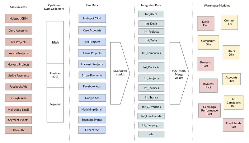
Data flows through the layers in the form of a dbt DAG (“Directed Acyclic Graph”) of data transformations:

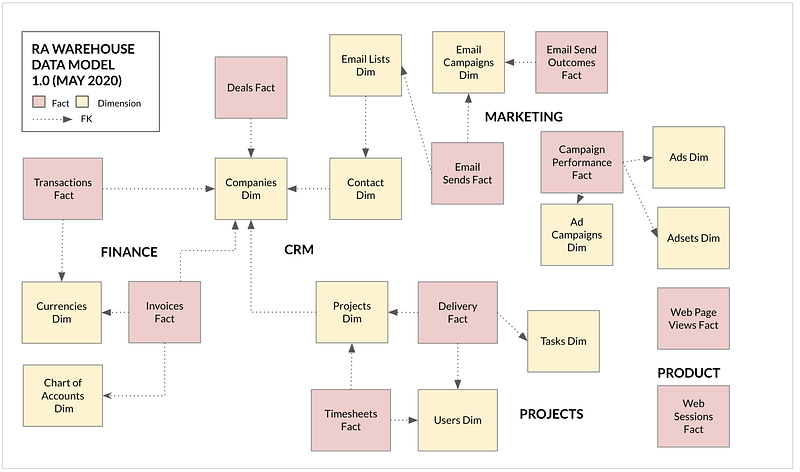
and populates a conformed, dimensional Kimball-style data warehouse.

How Do We Structure the dbt Project?

We’ve used a dbt project structure that looks like this:

├── analysis
├── data                      <-- "seed" files used for matching/merging companies, projects etc
├── macros
├── models
│   ├── integration           <-- "integration" models used to merge and dedupe models across multiple sources
│   ├── sources
│   │   ├── stg_asana_projects.        <-- "source" models with data-source specific transformations and
│   │   ├── stg_custom_source_1            renaming of columns into common formats. Where more than one
│   │   ├── stg_custom_source_2            pipeline technology (Stitch, Fivetran etc) is supported, these will
│   │   ├── stg_facebook_ads               contain SQL and jinja code for each pipeline type within the one model
│   │   ├── stg_gcp_billing_export         with the etl type configurable in the dbt_project.yml config file
│   │   ├── stg_google_ads
│   │   ├── stg_harvest_projects
│   │   ├── stg_hubspot_crm
│   │   ├── stg_intercom_messaging
│   │   ├── stg_jira_projects
│   │   ├── stg_mailchimp_email
│   │   ├── stg_mixpanel_events
│   │   ├── stg_segment_events
│   │   ├── stg_stripe_payments
│   │   ├── stg_unknown_values
│   │   └── stg_xero_accounting
│   ├── utils                           <-- "utils" models, for example for row count logging
│   └── warehouse                       <-- "warehouse" models containing fact and dimension tables,
│       ├── w_crm                           grouped by subject area
│       ├── w_finance
│       ├── w_marketing
│       └── w_projects

Each data source adapter loads the same columns in the same order for tables that are common to multiple sources, for example:

WITH source AS (
  {  }
  ),

renamed AS (
  SELECT
  concat('{  }',gid)           as user_id,
  name                   as user_name  ,
  email                  as user_email ,
  cast(null as boolean)         as user_is_contractor,
  case when email like '%@{  }%' then true else false end as user_is_staff,
  cast(null as int64)           as user_weekly_capacity,
  cast(null as string)          as user_phone,
  cast(null as int64)           as user_default_hourly_rate,
  cast(null as int64)           as user_cost_rate,
  true                          as user_is_active,
  cast(null as timestamp)       as user_created_ts,
  cast(null as timestamp)       as user_last_modified_ts
  FROM
    source
  WHERE
    name NOT LIKE 'Private User'
)
SELECT
  *
FROM
  renamed

Custom adapters are also provided to provide mappings into these common structures for one-off data sources specific to an implementation, i.e. a custom app database source.

What SaaS Sources and Warehouse Marts are Supported?

Right now, the RA Warehouse Framework supports the following SaaS data sources and pipeline technologies:

• Hubspot CRM (Stitch, Fivetran)
• Harvest Timesheets (Stitch)
• Xero Accounting (Stitch)
• Stripe Payments (Stitch)
• Asana Projects (Stitch)
• Jira Projects (Stitch)
• Mailchimp Email Marketing (Stitch)
• Segment Events (Segment)
• GCP Billing Exports
• Google Ads (Stitch)
• Facebook Ads (Stitch)
• Intercom Messaging (Stitch)
• Mixpanel Events (Stitch, Fivetran)
• Custom data sources

From these sources we currently load and populate the following warehouse “data marts”.

• Finance (Invoices, Chart of Accounts, Currencies)
• CRM (Deals, Contacts, Companies)
• Projects (Timesheet Projects, Timesheet Tasks, Delivery Projects, Delivery Tasks, Timesheets, Users)
• Marketing (Email lists, Email sends, Email campaigns, Ad Campaigns, Ad Performance, Web Page Views, Web Sessions)

Selectable and Configurable Data Sources

The particular data sources enabled for a warehouse implementation can be enabled or disabled by the setting of a flag in the dbt_project.yml configuration file, like this:

vars:
      enable_harvest_projects_source:      [true|false]
      enable_hubspot_crm_source:           [true|false]
      enable_asana_projects_source:        [true|false]
      enable_jira_projects_source:         [true|false]
      enable_stripe_payments_source:       [true|false]
      enable_xero_accounting_source:       [true|false]
      enable_mailchimp_email_source:       [true|false]
      enable_segment_events_source:        [true|false]
      enable_google_ads_source:            [true|false]
      enable_facebook_ads_source:          [true|false]
      enable_intercom_messaging_source:    [true|false]
      enable_custom_source_1:              [true|false]
      enable_custom_source_2:              [true|false]
      enable_mixpanel_events_source:       [true|false]
# warehouse modules
      enable_crm_warehouse:         [true|false]e
      enable_finance_warehouse:     [true|false]
      enable_projects_warehouse:    [true|false]
      enable_marketing_warehouse:   [true|false]
      enable_ads_warehouse:         [true|false]
      enable_product_warehouse:     [true|false]

Each data source then comes with its own model-scoped jinja variables that provide the schema and table names for each of the data source tables, in some cases let you switch between Fivetran, Stitch or Segment data pipelines and enable source-specific settings and choices:

stg_hubspot_crm:
              vars:
                  id-prefix: hubspot-
                  etl: stitch
                  stitch_companies_table: stitch_hubspot.companies
                  stitch_contacts_table: stitch_hubspot.contacts
                  stitch_deals_table: stitch_hubspot.deals
                  stitch_owners_table: stitch_hubspot.owners
                  stitch_pipeline_stages_table: stitch_hubspot.pipeline_stages
                  stitch_deal_pipelines_table: stitch_hubspot.deal_pipelines
                  fivetran_company_table: fivetran_hubspot_euwest2.company
                  fivetran_contact_table: fivetran_hubspot_euwest2.contact

Merging and Combining Dimensions Across Multiple Data Sources

Customers, contacts, projects and other shared dimensions are automatically created from all data sources, deduplicating by name and merge lookup files using a process that preserves source system keys whilst assigning a unique ID for each customer, contact etc.

Each set of model sources for a given dimension provide a unique ID, prefixed with the source name, and another field value (for example, user name) that can be used for deduplicating dimension members downstream. These fields are then initially merged (UNION ALL) together in the integration layer of the warehouse:

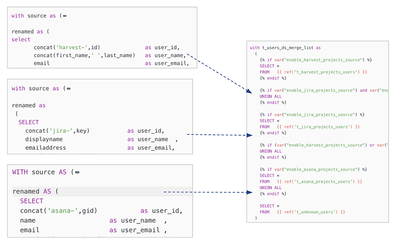
An CTE containing an array of source dimension IDs is then created within the int_ integration view, grouped by the deduplication column (in this example, user name). Any other multivalue columns are similarly-grouped by the deduplication column in further CTEs within the integration models, for example list of email addresses for a user.

user_emails as (
       SELECT user_name, array_agg(distinct lower(user_email) ignore nulls) as all_user_emails
       FROM t_users_merge_list
       group by 1),
 user_ids as (
       SELECT user_name, array_agg(user_id ignore nulls) as all_user_ids
       FROM t_users_merge_list
       group by 1)
 select i.all_user_ids,
        u.*,
        e.all_user_emails
       from (
select user_name,
...
FROM t_users_merge_list
group by 1) u
join user_emails e on u.user_name = coalesce(e.user_name,'Unknown')
join user_ids i on u.user_name = i.user_name

For dimensions where merging of members by name is not sufficient (for example, company names that cannot be relied on to always be spelt the same across all sources) we can add seed files to map one member to another and then extend the logic of the merge to make use of this merge file.

Within BigQuery these arrays of email addresses, user IDs and addresses are stored as nested, repeated groups of columns that maximise storage efficiency within BigQuery and are automatically “unravelled” when brought into Looker.

Data Profiling, ETL Results Reporting and Other dbt Macros

Finally, along with dbt schema and custom schema tests we make extensive use of macros to enable us to report on the outcome of each dbt Cloud job run and profile source and warehouse target tables and views.

For example, this macro calculates a set of useful column statistics all views and tables within a given BigQuery dataset:

{%- macro profile_schema(table_schema) -%}

{% set tables = dbt_utils.get_relations_by_prefix(table_schema, '') %}
SELECT column_stats.table_catalog,
       column_stats.table_schema,
       column_stats.table_name,
       column_stats.column_name,
       case when column_stats.pct_null <= .1 then 'NULL' else 'NOT NULL' end as recommended_nullable,
       case when column_stats.pct_null > 0 and column_stats.pct_null <= .1 then false else true end as is_recommended_nullable_compliant,
       case when column_stats.pct_unique >= .9 then 'UNIQUE' else 'NOT UNIQUE' end as recommended_unique_key,
       case when column_stats.pct_unique >= .9 and column_stats.pct_unique < 1 then false else true end as is_recommended_unique_key_compliant,
       column_metadata.* EXCEPT (table_catalog,
                       table_schema,
                       table_name,
                       column_name),
       column_stats.* EXCEPT (table_catalog,
                              table_schema,
                              table_name,
                              column_name)
FROM
(
{% for table in tables %}
  SELECT *
  FROM
(
  WITH
    `table` AS (SELECT * FROM {  } ),
    table_as_json AS (SELECT REGEXP_REPLACE(TO_JSON_STRING(t), r'^{|}$', '') AS ROW FROM `table` AS t ),
    pairs AS (SELECT REPLACE(column_name, '"', '') AS column_name, IF (SAFE_CAST(column_value AS STRING)='null',NULL, column_value) AS column_value
              FROM table_as_json,UNNEST(SPLIT(ROW, ',"')) AS z,UNNEST([SPLIT(z, ':')[SAFE_OFFSET(0)]]) AS column_name,UNNEST([SPLIT(z, ':')[SAFE_OFFSET(1)]]) AS column_value ),
    profile AS (
    SELECT
      split(replace('{  }','`',''),'.' )[safe_offset(0)] as table_catalog,
      split(replace('{  }','`',''),'.' )[safe_offset(1)] as table_schema,
      split(replace('{  }','`',''),'.' )[safe_offset(2)] as table_name,
      column_name,
      COUNT(*) AS table_rows,
      COUNT(DISTINCT column_value) AS _distinct_values,
      safe_divide(COUNT(DISTINCT column_value),COUNT(*)) AS pct_unique,
      COUNTIF(column_value IS NULL) AS _nulls,
      COUNTIF(column_value IS NOT NULL) AS _non_nulls,
      COUNTIF(column_value IS NULL) / COUNT(*) AS pct_null,
      min(column_value) as _min_value,
      max(column_value) as _max_value,
      avg(SAFE_CAST(column_value AS numeric)) as _avg_value,
      APPROX_TOP_COUNT(column_value, 1)[OFFSET(0)] AS _most_frequent_value,
      MIN(LENGTH(SAFE_CAST(column_value AS STRING))) AS _min_length,
      MAX(LENGTH(SAFE_CAST(column_value AS STRING))) AS _max_length,
      ROUND(AVG(LENGTH(SAFE_CAST(column_value AS STRING)))) AS _avr_length
    FROM
      pairs
    WHERE
      column_name <> ''
      AND column_name NOT LIKE '%-%'
    GROUP BY
      column_name
    ORDER BY
      column_name)
  SELECT
    *
  FROM
    profile)
{%- if not loop.last %}
    UNION ALL
{%- endif %}
{% endfor %}
) column_stats
LEFT OUTER JOIN
(
  SELECT
    * EXCEPT
      (is_generated,
       generation_expression,
       is_stored,
       is_updatable)
  FROM
    {  }.INFORMATION_SCHEMA.COLUMNS
) column_metadata
ON  column_stats.table_catalog = column_metadata.table_catalog
AND column_stats.table_schema = column_metadata.table_schema
AND column_stats.table_name = column_metadata.table_name
AND column_stats.column_name = column_metadata.column_name

{%- endmacro -%}

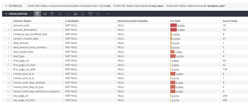
Then, combined with a data visualization in Looker, we can quickly identify those table columns that are nearly unique or not null so that we can focus our time on addressing what are probably data errors in the rows that aren’t unique or contain null values.

What Features and Other Support are on the Product Roadmap?

High-priority features we plan to add in the very near future include:

• Extending Fivetran support to cover all remaining data source types
• Add more support for incremental loading of warehouse tables
• Complete test coverage of warehouse and integration layer models

Medium-priority are:

• Extending Segment support to cover all appropriate remaining data sources
• Snowflake as an alternative to Google BigQuery as the warehouse platform
• Enrichment plugins, e.g. Clearbit

Help Build The Missing Layer in the Modern BI Stack

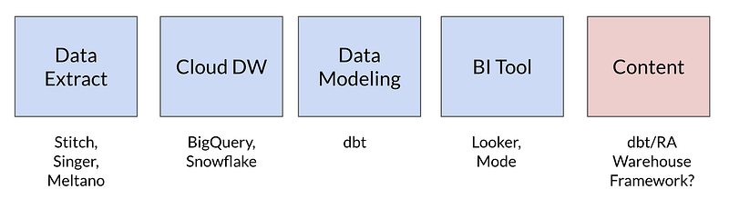
Community Contributions are welcome, and in-fact we’re hoping this project might in-time become an open-source “content and data warehousing” layer on-top of dbt, filling in the missing layer in the open-source modern BI stack that we felt was missing until now.

How Do I Find Out More?

The RA Warehouse dbt package is now up on Github as a public repo, and feel free to email us at info@rittmananalytics.com for more information … or if you’d like us to bring this framework and our data centralization services to your organization.

First published on the Rittman Analytics blog on 28th May 2020.

Recent Posts

RSS Feed

Published Year

Tag Cloud